Field note
ch16
Query Optimization
Outline:
- Introduction
- Transformation of Relational Expressions
- Statistical Information for Cost Estimation
- Cost-based Optimization
- Dynamic Programming for Choosing Evaluation Plans
- Nested Subqueries
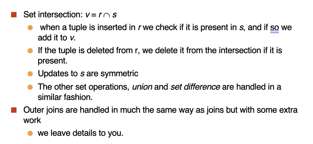
- Materialized Views
- Advanced Topics in Query Optimization
Introduction
-
Alternative ways of evaluating a given query
- Equivalent expressions
- 逻辑优化, transformation based optimization
- Different algorithms for each operation
- 物理优化, cost based optimization
- Equivalent expressions
-
Estimation of plan cost based on:
- Statistical information about relations. Examples:
- number of tuples, number of distinct values for an attribute
- Statistics estimation for intermediate results(Cardinality Estimation)
- to compute cost of complex expressions
- Cost formulae for algorithms, computed using statistics
- Statistical information about relations. Examples:
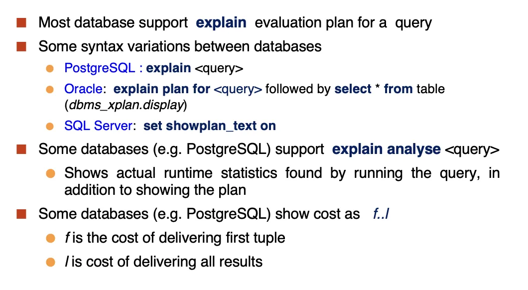
Viewing Query Evaluation Plans
如果想要查看数据库系统选择的查询计划,可以使用 EXPLAIN 语句。这个语句会显示出数据库系统在执行查询时所选择的查询计划,包括每个操作的成本估计和执行顺序。
Transformation of Relational Expressions
- Two relational algebra expressions are said to be equivalent if the two expressions generate the same set of tuples on every legal database instance.
- 如果两个关系代数表达式在每个合法的数据库实例上生成相同的元组集合,则这两个表达式是等价的。
- An equivalence says that expressions of two forms are equivalent.
- Can replace expression of first form by second, or vice versa
Equivalence Rules
Selection Operations
- Conjunctive selection operations can be deconstructed into a sequence of individual selections.选择操作可以分解为一系列单独的选择操作。
- Selection operations are commutative.选择操作是可交换的。
- Only the last in a sequence of projection operations is needed, the others can be omitted.投影操作中只有最后一个是必要的,其他的可以省略。
-
Selections can be combined with Cartesian products and theta joins.选择操作可以与笛卡尔积和 连接结合使用。
a.
b.
-
Theta-join operations (and natural joins) are commutative. 连接操作(和自然连接)是可交换的。
- (a). Natural join operations are associative.自然连接操作是结合的。
- (b). Theta joins are associative in the following manner:
: where involves attributes from only and
-
The selection operation distributes over the theta join operation under the following two conditions
a. When all the attributes in involve only the attribute of one of the expressions() begin joined.
b. When involves only the attributes of and involves only the attributes of .
Projection Operations
The projection operation distributes over the theta join operation as follows:
a. if involves only attributes from :
b. Consider a join .
- Let and be sets of attributes from and , respectively.
- Let be attributes of that are involved in join condition , but are not in and
- Let be attributes of that are involved in join condition , but are not in .
Set Operations
- The set operations union and intersection are commutative
- Set union and intersection are associative
- The selection operation distributes over and operations as follows:
also: and similarly for in place of , but not for .
- The projection operation distributes over union
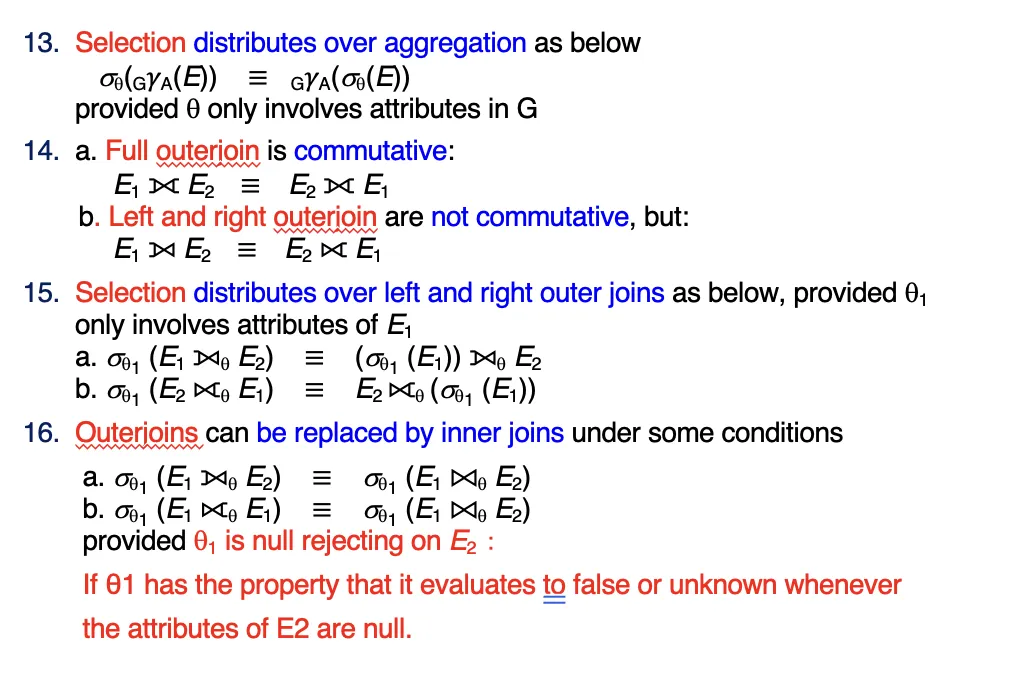
Other Equivalence Rules
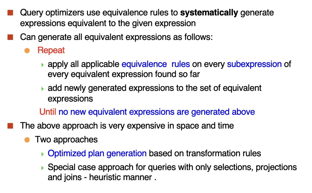
Enumeration of Equivalent Expressions
Statistics for Cost Estimation
估计代价需要以下的信息:
- : number of tuples in a relation .
- : number of blocks containing tuples of .
- : size of a tuple of .
- : blocking factor of - i.e., the number of tuples of that fit into ont block.每个块能放几个元组
- : number of distinct values that appear in for attribute ; same as the size of .
- If tuples of are stored together physically in a file, then:
Selection Size Estimation
-
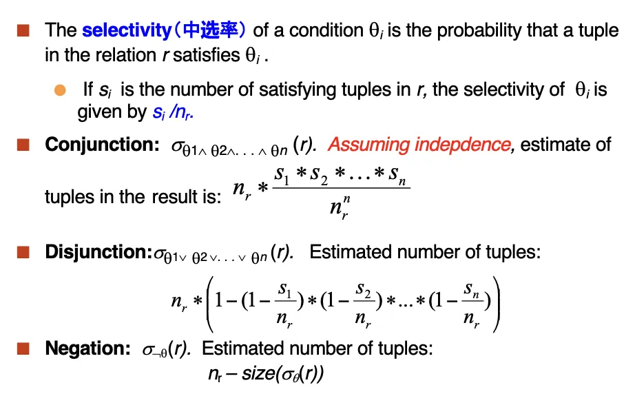
- : number of records that will satisfy the selection
- Equality condition on a key attribute: size estimate = 1
-
- Let c denote the estimated number of tuples satisfying the condition.
- If min(A, r) and max(A, r) are available in catalog
- c = 0 if
- c =
- If histograms available, can refine above estimate
- In absence of statistical information c is assumed to be .
Join Size Estimation
The Cartesian product contains tuples; each tuple occupies bytes.
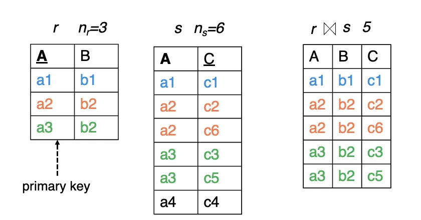
- If , then is the same as
- If is a key for , then a tuple of s will join at most one tuple from .
- Therefore, (the number of tuples in )
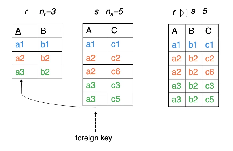
- If is a foreign key in referencing , then the number of tuples in
- The case for being a foreign key referencing is symmetric.
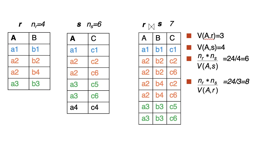
- If is not a key for or
- If we assume that every tuple in produces tuples in , the number of tuples in is estimated to be:
可以理解为:每一个 都可以和 中的每一个元组进行连接.
: If the reverse is true, the estimate obtained will be:
Size Estimation for Other Operations
- Projection: estimated size of
- Aggregation: estimated size of $$_A\mathcal{G}(r) = V(A, r)$
- Set operations:
- For unions/intersections of selections on the same relation: rewrite and use size estimate for selections
- E.g., can be rewritten as
- For operations on different realtions:
- Estimated size of = size of + size of
- Estimated size of = min(size of , size of )
- Estimated size of = size of
- All the three estimated may be quite inaccurate, but provide upper bounds on the sizes.
- For unions/intersections of selections on the same relation: rewrite and use size estimate for selections
- Outer join:

Estimation of Number of Distinct Values
- Selections: , estimate
- If forces A to take a specified value:
- e.g., A = 3
- If forces A to take on one of a specified set of values:
- e.g., A in {1, 2, 3}
- If the selection condition is of the form , estimated
- Where is the selectivity of the selection
- In all the other cases, use approximate estimate:
- If forces A to take a specified value:
- Joins: , estimate
- If all attributes in A are from , the estimated
: - If A contains attributes A1 from and A2 from , then estimated
Choice of Evaluation Plans
Cost-based Join-Order Selection
Consider finding the best join-order for
There are different join orders for above expression.
!!! EXAMPLE
Join Order Optimization Algorithm
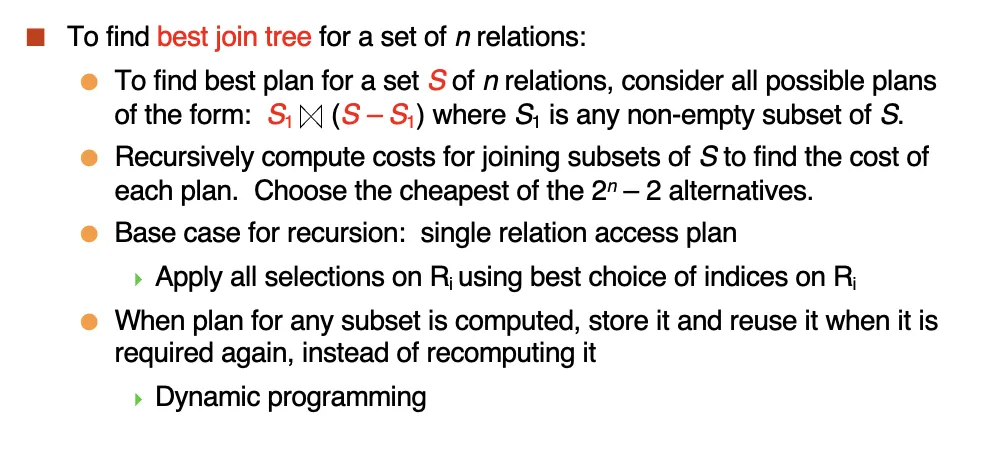
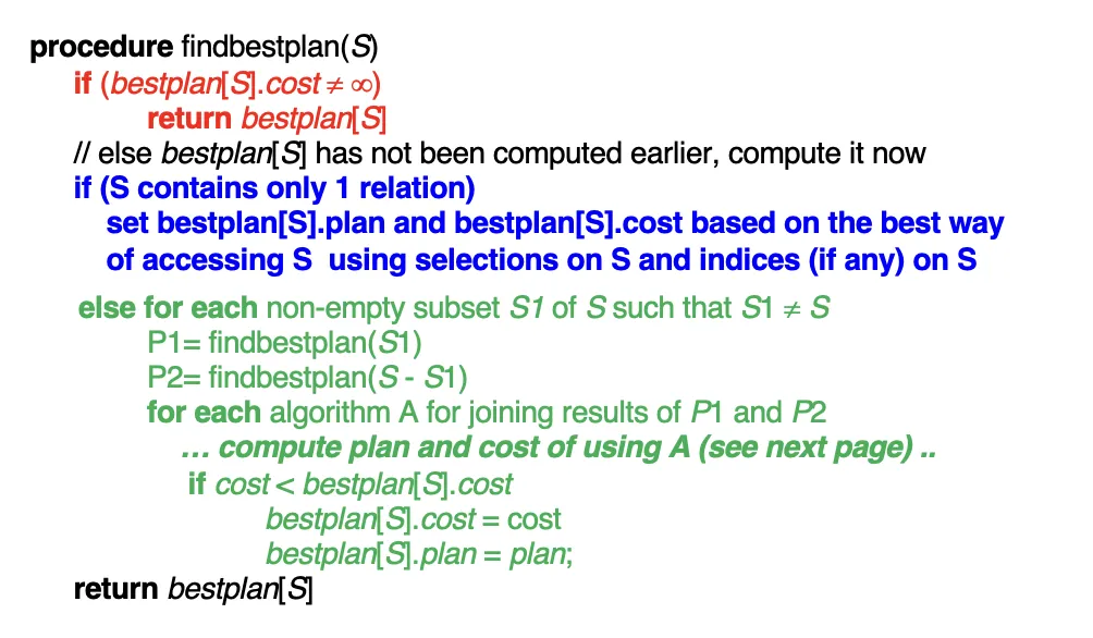
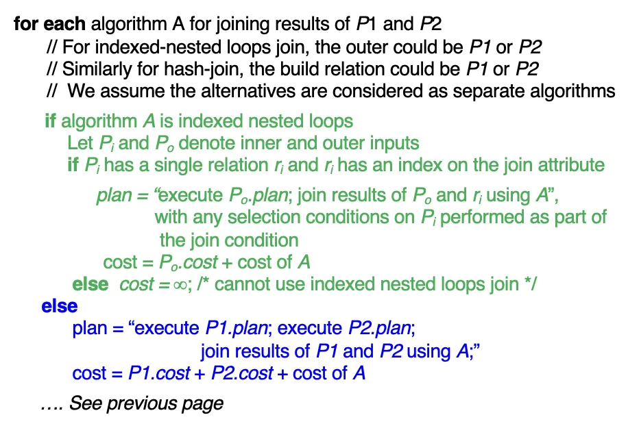
- 对于一个集合 , 考虑其所有形式为 的连接方案,其中 是 的一个子集。
- 对于 的每一个子集,递归计算其连接方案的代价。
- 当递归到单个关系时,考虑对其采取所有的连接方案,从而找出最优的连接方案。
- 实际上是一个动态规划的思想。
Left Deep Join Trees
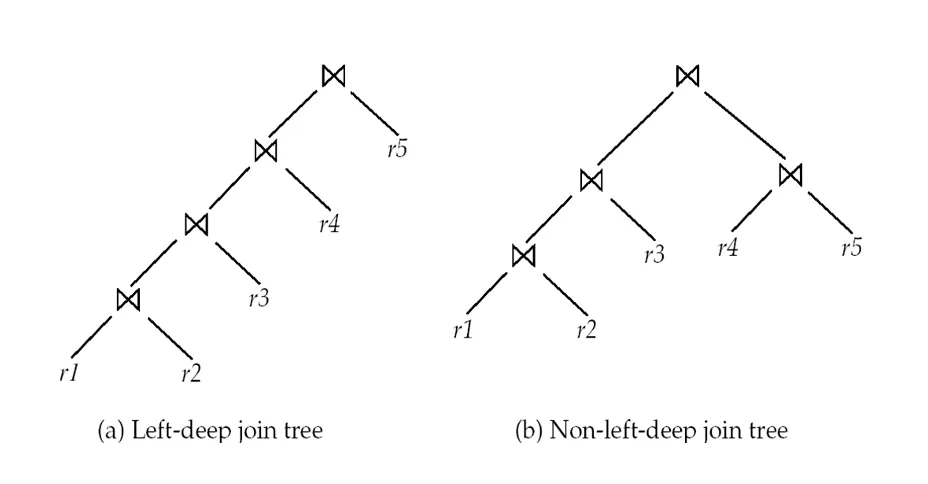
In left-deep join trees, the right-hand-side input for each join is a relation, not the result of an intermediate join.
在 left-deep-join trees 中,每个连接的右侧输入都是一个关系,而不是中间连接的结果。
左边可以是中间结果。
Cost of Optimization
- With dynamic programming
- Time complexity of optimization with bushy tree is
- Space complexity is
- If only left-deep trees are considered
- Time complexity of finding best join order is
- Space complexity is
Heuristic Optimization(启发式优化)
- Systems may use Heuristics to reduce the number of choices that must be made in a cost-based fashion.
- Heuristic optimization transforms the query-tree by using a set of rules that typically (but not in all cases) improve execution preformance:
- Perform selection early(reduces the number of tuples)
- Perform projection early(reduces the number of attributes)
- Perform most restrictive selection and join operations(i.e. with smallest result size) before other similar operations.
- Perform left-deep join order
Additional Optimization Techniques
Nested Subqueries
- Nested query example:
select name
from instructor
where exists (select *
            from teaches
where instructor.ID = teaches.ID and teaches.year = 2022)- SQL conceptually treats nested subqueries in the where clause as functions that take parameters and return a single value or set of values.
- Parameters are variables from outer level query that are used in the nested subquery; such variables are called correlated variables(相关变量).
在上边的例子中,对于每一层外部循环,我们都要遍历内层的循环。但是如果来自外循环的变量没有相关变量的话,那么我们可以先执行内层的循环,然后将结果传递给外层的循环。
- The semijoin(半连接) operator ⋉ is defined as follows:
- If a tuple appears times in , it appears times in the result of , if there is at least one tuple in matching with .
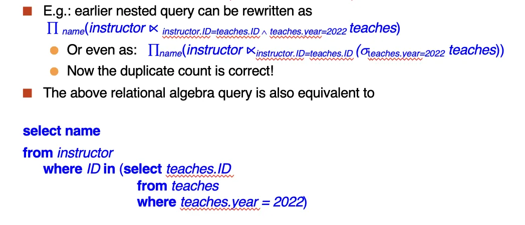
- The process of replacing a nested query by a query with a join/semijoin (possibly with a temporary relation) is called decorrelation(去除相关).
Decorrelation
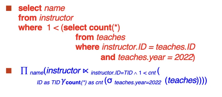
- Decorrelation of scalar aggregate subqueries can be done using groupby/aggregation in some cases.
Materialized Views
- A materialized view is a view whose contents are computed and stored.
create view department_total_salary(dept_name, total_salary) as
select dept_name, sum(salary)
from instructor
group by dept_name
Materialized View Maintenance
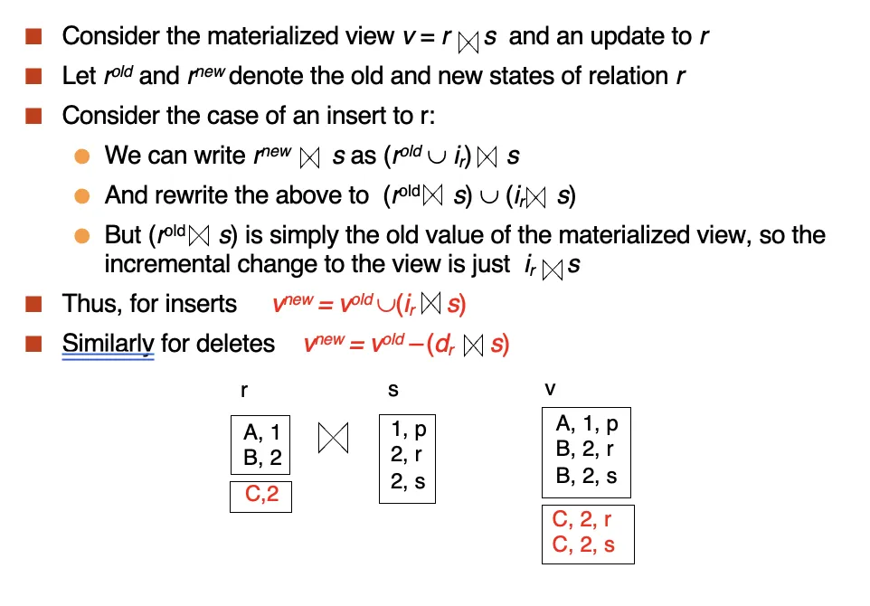
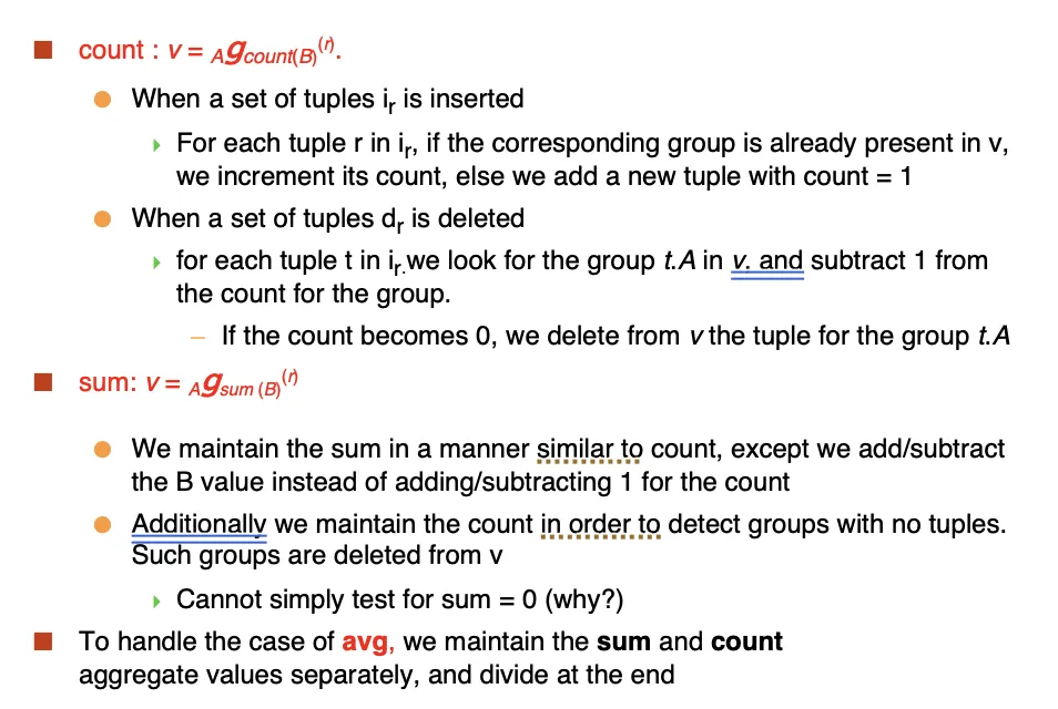
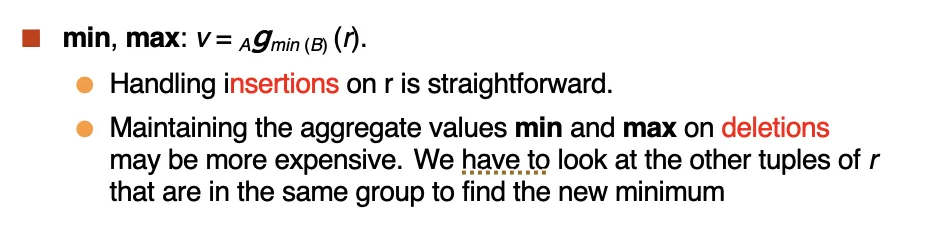
Use incremental maintenance(增量视图维护).
Changes to database relations are used to compute changes to the materialized view, which is then updated.
对于数据库的关系的变化,我们可以计算出物化视图的变化,然后更新物化视图。
The changes (inserts and deletes) to a relation or expressions are referred to as its differential(差分).
Join Operation
Selection and Projection Operations
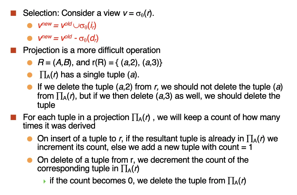
Seelction: Consider a view
: - : -
Aggregation Operations
Other Operations