Field note
ch2
Pipeline
What is Pipeline
Three modes of execution:
- Sequential execution
- Single overlapping execution
- Twice overlapping execution
假设指令的执行被分为三个阶段:
- Instruction fetch (IF)
- Instruction decode (ID)
- Execute (EX)
Sequential execution
如果指令是顺序执行的话,只能等上一条指令执行结束后,才能执行下一条指令。
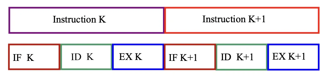
那么总的执行时间
Overlapping execution
每一条指令内部是顺序执行的,但是不同指令之间可以重叠执行。
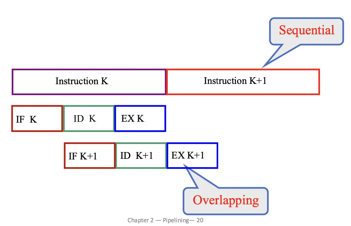
上图是每个阶段时间相同,每个阶段可以很好的重叠执行。
但是,如果每个阶段时间不同的话,就会发生资源的浪费,比如:
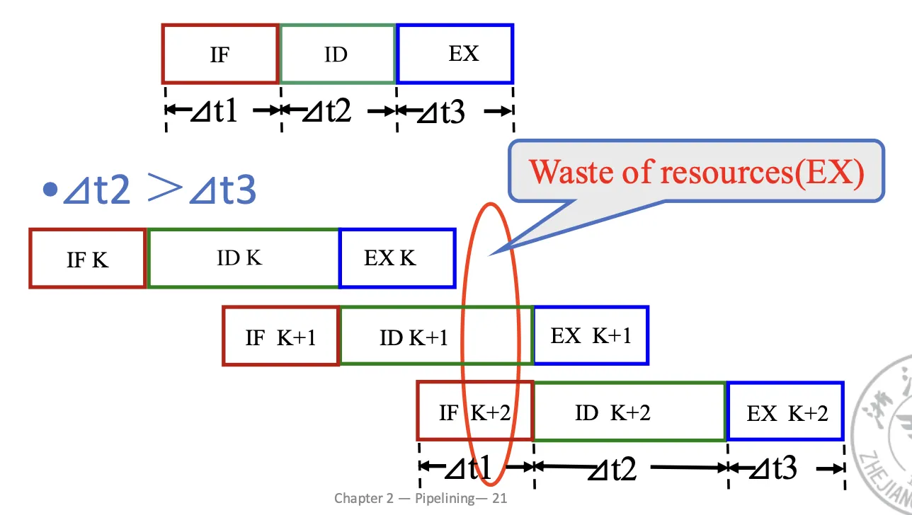
或者:
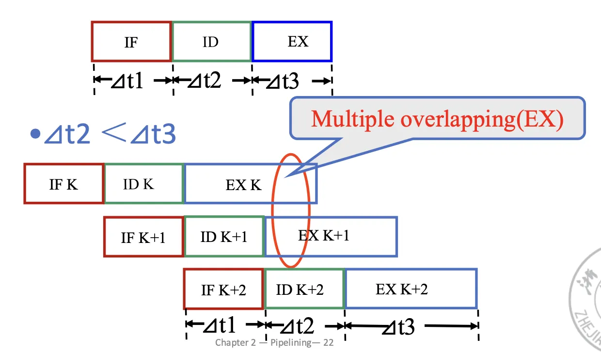
-
Single overlapping execution : 可以缩短的时间,但是需要额外的硬件开销
条指令总的执行时间:
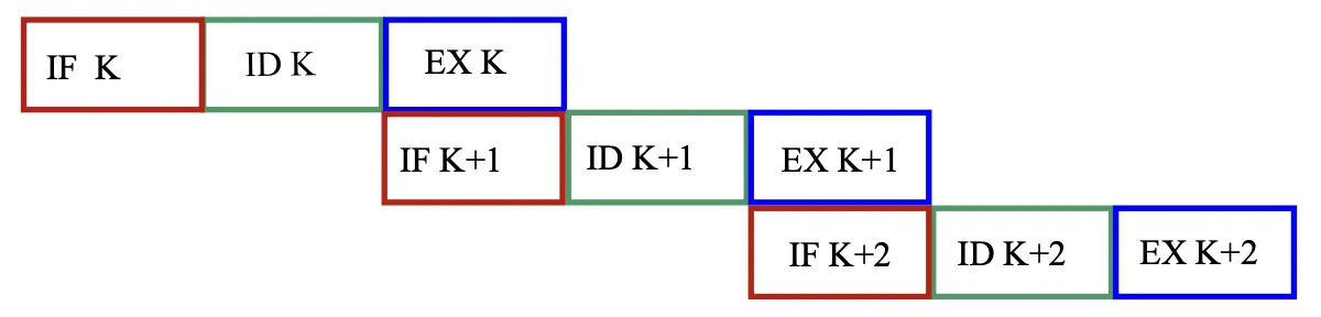
-
Twice overlapping execution : 可以缩短的时间,但是需要更多的硬件开销,并且需要另外的 FETCH, DECODE, EXECUTE 插件。
条指令总的执行时间:
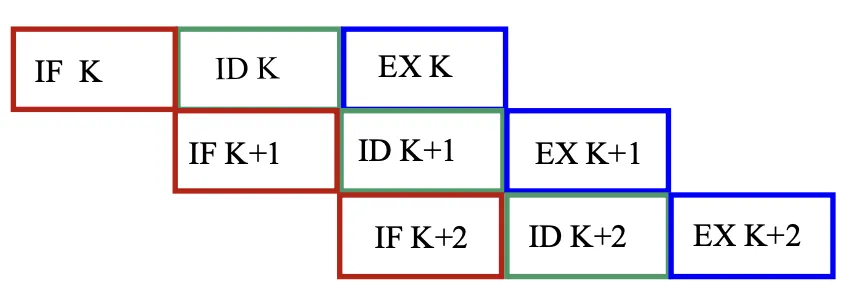
Adding Instruction Buffer
Conflict in access memory:
- Instruction memory & data memory
- Instruction cache & data cache (same memory):Harvard architecture
- Multibody cross structure (same memory with limitations)
- Adding instruction buffer between instruction memory and instruction decode unit
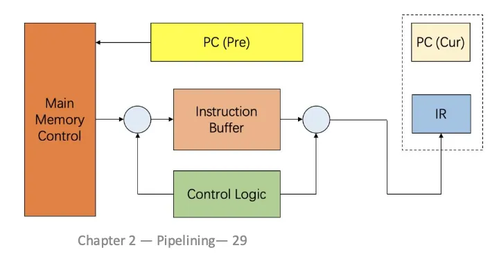
在取指和内存中间加上一个 buffer ,只要这个 buffer 没满,就一直取指令。
添加 buffer 之后,取指的时间变得非常短,因此可以把 IF 和 ID 两个阶段合并,这样 Twice overlapping 就变成了 Single overlapping。
但是如果合并后的 ID 阶段执行时间和 EX 阶段执行时间不同的话,就会浪费资源。
Advanced Control
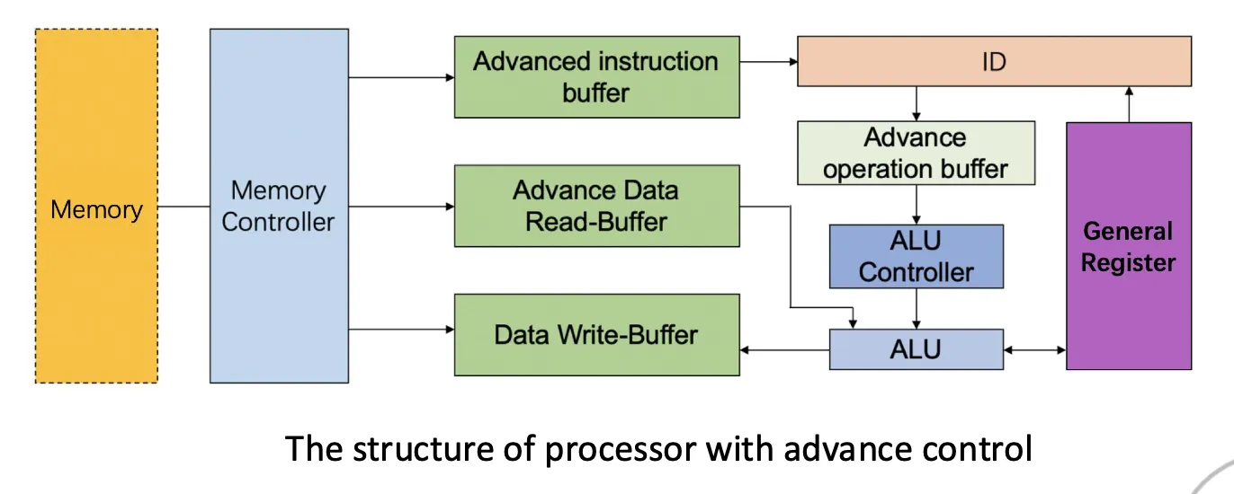
可以把 ID 阶段提前执行,然后把结果存到 buffer 中,等到 EX 阶段执行的时候再取出来。
Common features: They work by FIFO, and are composed of a group of serveral storage units that can be accessed quickly and related control logic.
通过 FIFO(先进先出)等方式,提高了指令的执行效率。
Classes of Pipeline
- Single function pipeline: only the fixed function pipelining.
- Multi function pipelining: each section of the pipelining can be connected differently for serveral different functions.
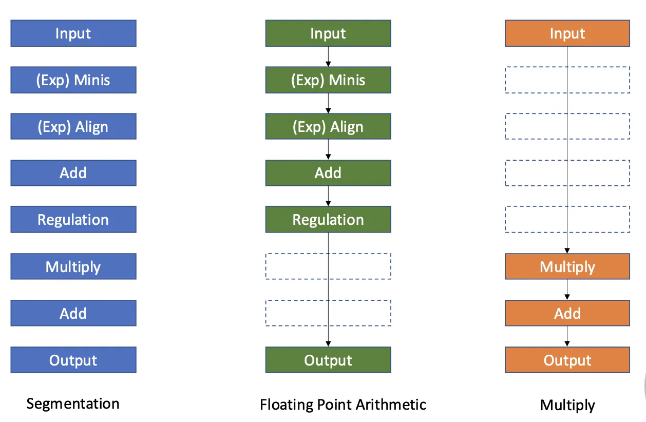
上图中左侧 Segmentation 表示流水线中所有的元件,中间的 FLoating Point Arithmetic 表示浮点运算需要的元件,右侧的 Multiply 表示乘法需要的元件。
而对于 Multi function pipelining,又可以分为两类:
- Static pipelining(静态流水线): 在同一时间,流水线的每个部分只能执行相同类型的操作 这就意味着对于静态流水线,只有输入的是相同类型的指令,它的效率才能最大化。
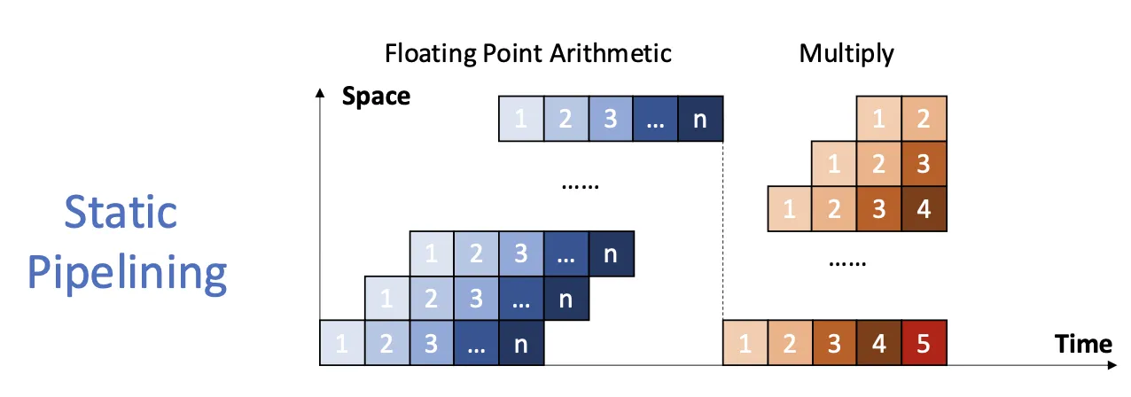
从上图可以看出,对于 Floating Point Arithmetic 和 Multiply 部分,静态流水线只能等 Floating Point Arithmetic 部分执行完毕后,才能执行 Multiply 部分。
- Dynamic pipelining(动态流水线): 在同一时间,流水线的每个部分可以执行不同类型的操作
- 灵活,但是控制信号复杂
- 提高单元的利用率
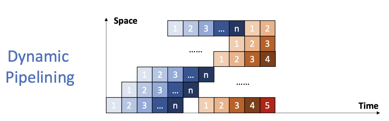
不同于静态流水线,动态流水线可以在同一时间执行不同类型的操作。
根据粒度分类:
- Component level pipelining(组件级流水线): 处理器的算数和逻辑组件分成很多段,从而不同种类的操作都可以执行
- Processor level pipelining: 指令的解释和执行是通过流水线实现的。指令的执行过程被分成很多小部分,每个小部分都是通过独立的功能模块实现的。
- Inter processor pipelining: 由一系列的处理器串联组成,每个处理器执行一个指令的一个部分,然后把结果传递给下一个处理器。
根据是否线性分类:
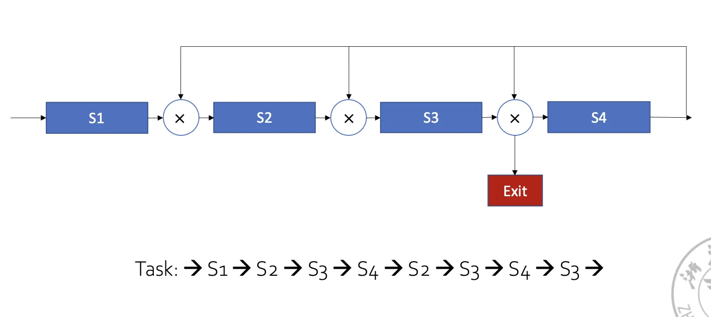
- Linear pipelining: 流水线每个部分串联,没有反馈回路。数据最多流过每个部分一次。
- Nonlinear pipelining: 串行连接,并且存在反馈回路。
分为顺序/乱序:
- Ordered pipelining: 在流水线中,任务输出顺序与输入顺序完全相同,每个任务按顺序流过流水线。
- Disordered pipelining: 任务的输出顺序与输入顺序不同,允许后边的任务先完成。
根据是否能处理向量数据分类:
- Scalar pipelining: 流水线没有向量处理程序,只能处理标量数据。
- Vector pipelining: 流水线可以处理向量数据。
Pipeline Performance
Throughput(TP)
TP: 每个时钟周期可以完成的指令数
: 完成的指令数 : 完成所有指令所用的时间
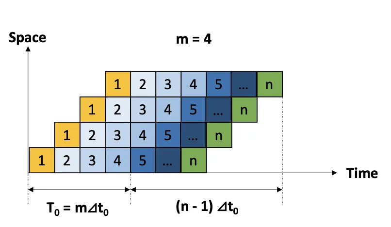
当 很大,即指令很多时, 可以近似为:
就是说流水线的吞吐量只与时钟周期有关,与流水线的级数无关。
那么
如果流水线每个阶段的时间不一样的话,我们把最长的那个阶段叫做 bottleneck stage(瓶颈阶段).
那么
可以看到, 只与瓶颈阶段时间有关。
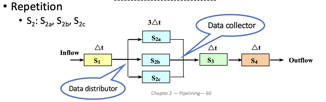
Common methods to solve pipeline bottleneck
- Subdivision: 把瓶颈阶段分成几个小阶段,每个阶段时间与其他阶段相等,都是。

- Repetition: 在瓶颈阶段多用几个部件,这样就可以提高吞吐量。
Speedup(Sp)
Speedup(加速比): 一个流水线相对于一个非流水线的性能提升。
如果 ,那么 。
Efficiency
Efficiency(效率): 从计算机硬件考虑,纵轴代表使用不同的部件,效率指的是我们真正使用这个部件占整个时空的百分比。
总空间为 ,因为一共有个部件,每个部件有个时空。
指令占的空间为 。一共个指令,每个指令占个时空。
则效率
若 ,那么 。
!!! question
=== "Static pipeline"
<font figure markdown="span">

</font>
注意到这里是<font color = red>静态双功能流水线</font>,必须在乘法做完之后才能做加法。

所以:
$$
TP = \frac{4 + 3}{15}\Delta t = \frac{7}{15}\Delta t
$$
$$
Sp = \frac{4 \times 3\Delta t + 3 \times 4\Delta t}{15\Delta t} = 1.6
$$
$$
\eta = \frac{3 \times 4\Delta t + 4 \times 3\Delta t}{4 \times 3\Delta t} = 32%
$$
=== "Dynamic pipeline"
<font figure markdown="span">

</font>
注意到这里是<font color = red>动态双功能流水线</font>,可以在乘法做的同时做加法。

既然流水线这么好,那么我们是不是可以把流水线的级数无限加大呢?
实则不然,太多的级数会导致:
- Lots of complications,太复杂了
- 大量的指令同时进行,中间可能存在复杂的依赖关系
- 控制信号太多了
- 需要特别多的流水线寄存器,硬件开销太大
Hazards of Pipeline
更详细的笔记请看计组部分的笔记。
Hazards
- Situations that prevent starting the next instruction in the next cycle
- Structure hazards
- A required resource is busy
- Data hazard
- Need to wait for previous instruction to complete its data read/write
- Control hazard
- Deciding on control action depends on previous instruction
Structure Hazards
对于流水线中结构的冲突
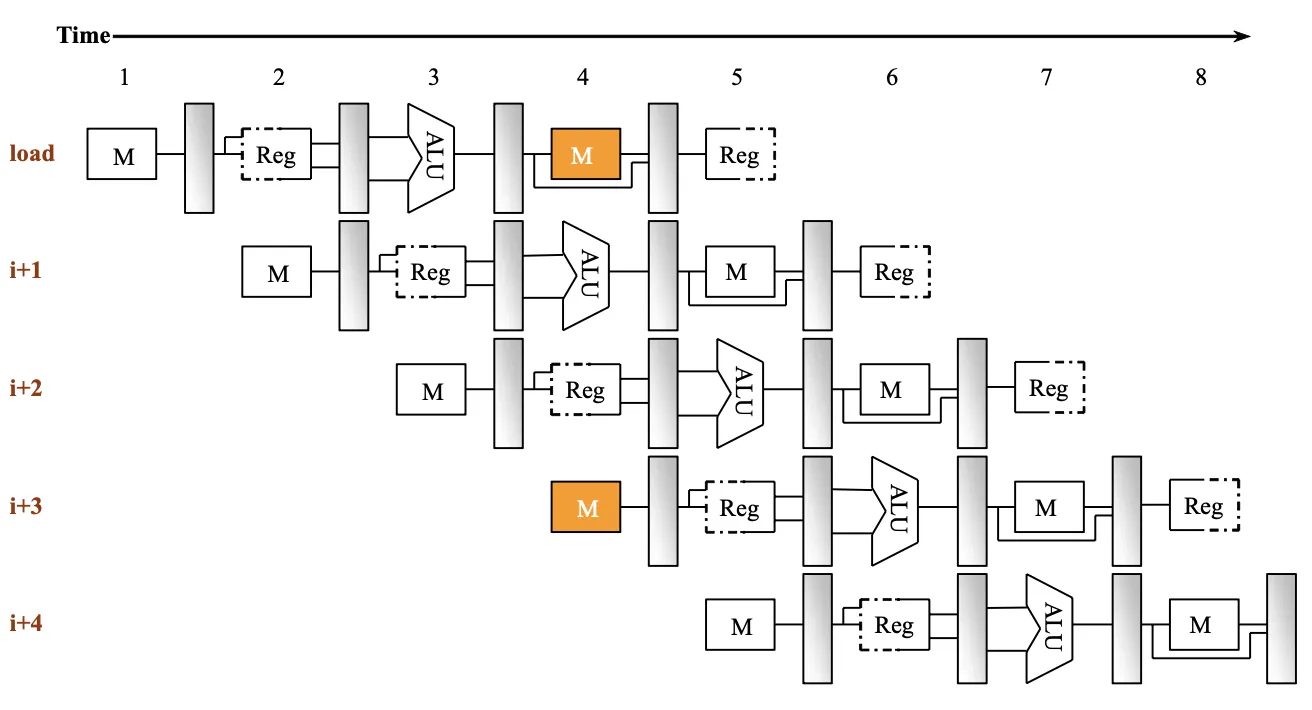
上图就是流水线中发生了对 memory 对冲突。
对于结构冲突,一般通过加 bubble 或者硬件的方式解决。
Data Hazards
An instruction depends on completion of data access by a previous instruction
- Read after write(RAW).可以通过 forwarding 解决
FADD.D f6, f0, f12
FSUB.D f8, f6, f14- Write after read(WAR)
FDIV.D f2, f6, f4
FADD.D f6, f0, f12- Write after write(WAW)
FDIV.D f2, f0, f4
FSUB.D f2, f6, f14
但是并不是所有的 RAW 都可以通过 forwarding 解决,比如 load-use hazard.
这时候需要在 load 指令后边加一个 bubble, 然后才能 进行 forwarding.
Control Hazards
- Conditional jump: branch
- Unconditional jump: jal, jalr
为了减少分支带来的影响,可以采用预测分支的方式。
- Static branch prediction
- Always taken
- Always not taken
- Delayed branch
- Dynamic branch prediction
Control Hazards
Static Branch Prediction
- Always taken: 永远预测分支会发生
- Always not taken: 永远预测分支不会发生
- Delayed branch: 延时槽
不论我是否跳转,有些指令是一定会执行的,可以把这些指令放在延时槽中。
Dynamic Branch Prediction
Use dynamic prediction
- Branch prediction buffer (aka branch history table)
- Indexed by recent branch instruction addresses
- Stores outcome (taken/not taken)
- To execute a branch
- Check table, except the same outcome: 把之前的所有跳转结果都记录下来,根据之前的结果预测这次的结果。
- Start fetching from fall-through or target: 根据预测的结果,开始取指。
- If wrong, flush pipeline and flip prediction: 如果预测错误,就把之前的指令都清空,重新开始。
Branch History Table(BHT)
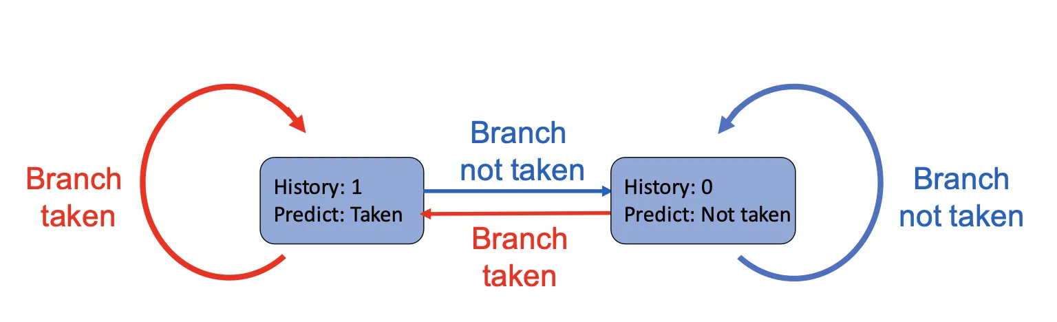
实际上是一个有限状态机的模式,根据前边的结果,预测后边的结果。
我们有 1-bit predictor 和 2-bit predictor。
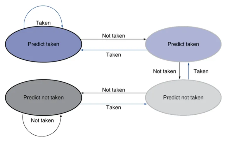
Advanced Techniques for Instruction Delivery and Speculation
- Increasing Instruction Fetch Bandwidth
- Branch-Target Buffers
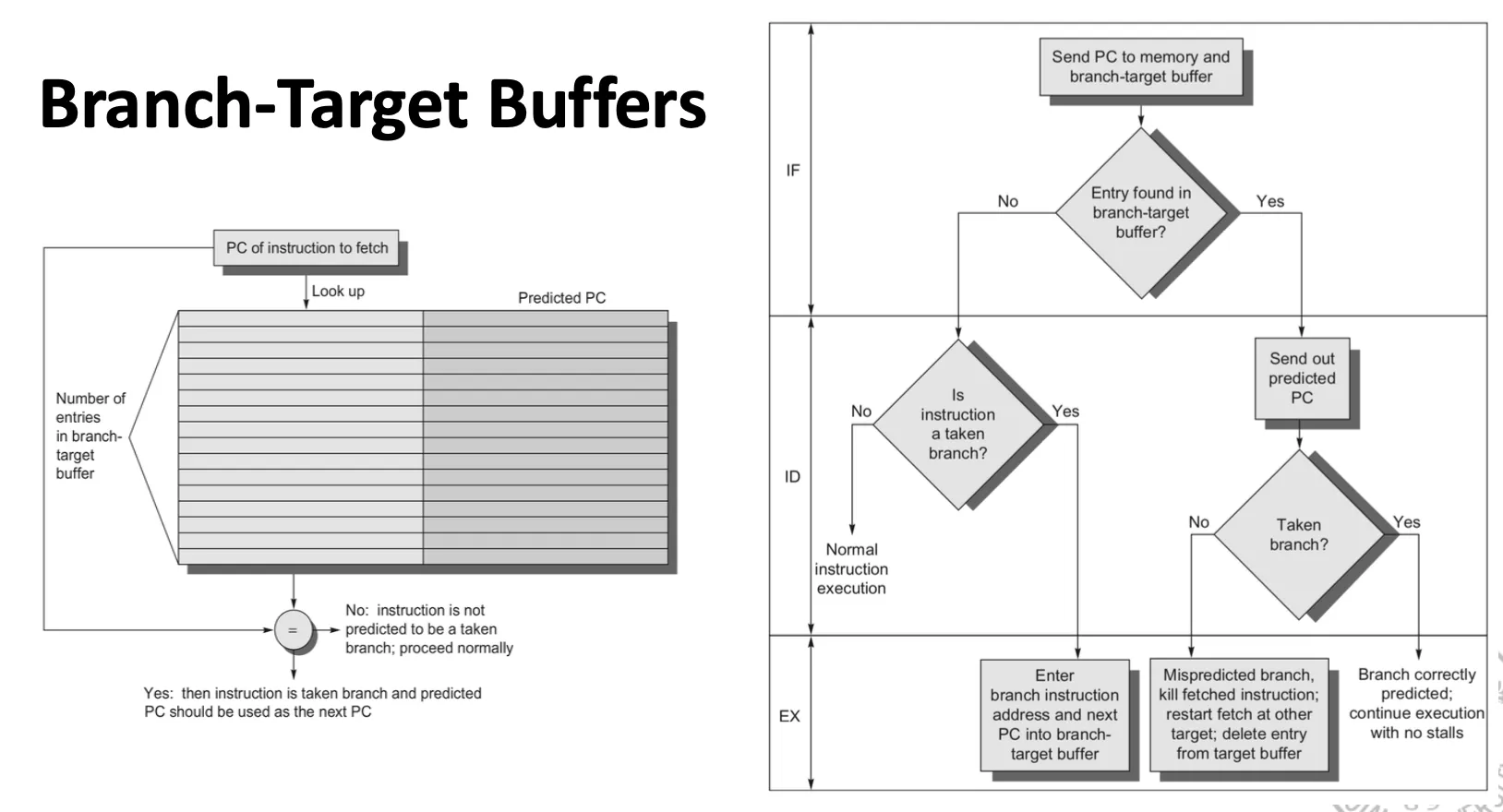
类似于 TLB , 存放的是跳转的目标地址,如果跳转的分支指令在 BTB 中,就可以直接取出目标地址;如果不跳转的话,就直接把地址去掉。
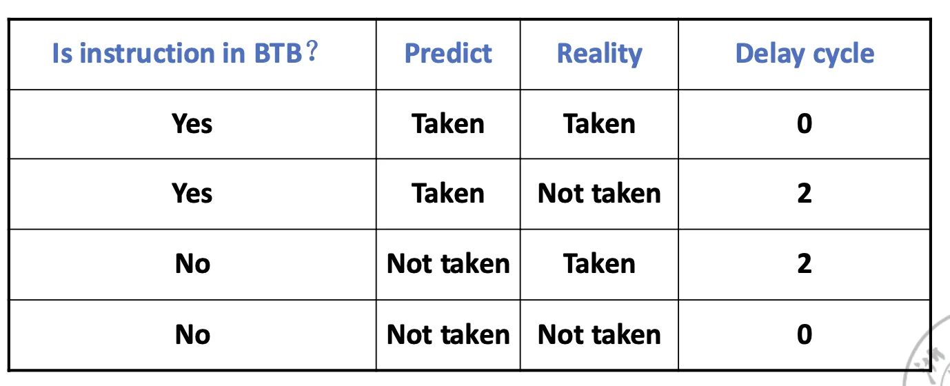
- Specialized Branch Predictors: Predicting Procedure Returns, Indirect Jumps, and Loop Branches
- Integrated Instruction Fetch Units
BTB Cache 的优势:
- 更快地取指
- 可以在分支目标处一次提供多个指令,在多处理器中很有用
- branch folding: 可以在不延迟的情况下实现无条件跳转,或有条件跳转
Schedule of Nonlinear Pipeline
Nonlinear pipeline: In addition to the serial connection, there is also a feedback loop in the pipeline.
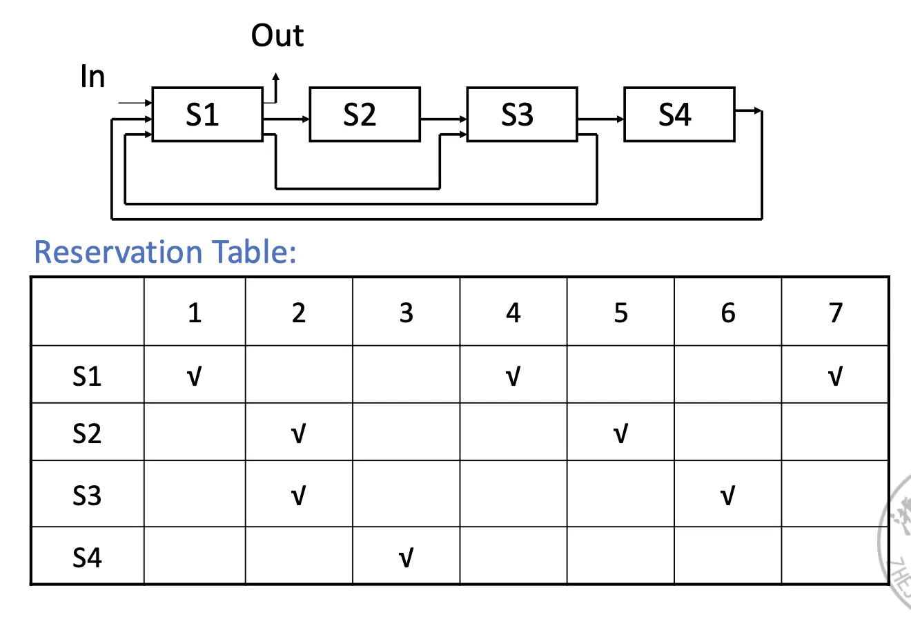
如上图中的非线性流水线,我们可以用一个表来表示元件的占用情况,其中横轴的数字表示拍数(第几拍),纵轴表示元件的编号。
如何进行规划?
- Initial Conflict Vertor: 初始冲突向量,二进制表示
- Conflict Vector
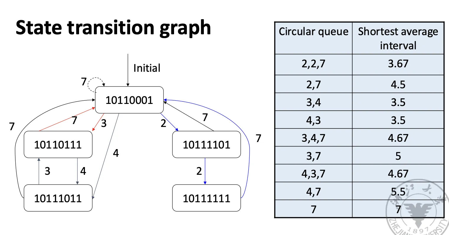
- State transition graph
- Circular queue
- Shortest average interval
首先确定初始冲突向量
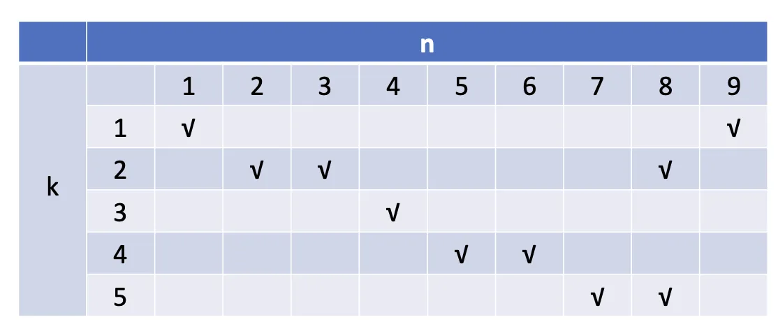
表的结构与之前说的相同,我们需要做的就是如果第 拍需要用到元件 , 就在对应位置打勾。
然后就是确定各个部件的冲突情况。从上图中可以看出,元件 1 在第 1 和 9 拍会产生冲突,中间隔了 8 拍。
元件 2 在第 2,3,8 拍产生冲突,中间隔了 拍。
其他元件类似。所以我们就得到了总第间隔拍数。
那么将对应二进制位(1,5,6,8)置为 1,得到冲突向量(从右向左)。
然后确定冲突向量
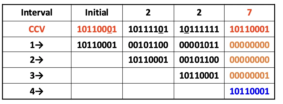
横轴的数字 2, 2, 7表示隔几拍进下一条指令,我们相应就把冲突向量右移 2, 2, 7 位,然后和本来的冲突向量或运算,得到新的冲突向量。
这里纵轴的”1->” , “2->” 表示右移多少次。
我们发现,循环调度 2-2-7 可以让冲突向量回到最初状态,说明我们找到了一个循环调度。